The optimal investment problem in Antares-Xpansion¶

General description¶

Antares-Xpansion minimizes the following cost:

$$ \min (\text{expected operating costs for one year} + \text{fixed cost annuity}) $$ over a set of investment variables specified by the user.

The expected operating costs for one year, calculated by Antares, includes the variable costs of thermal generation (fuel and CO2 costs), penalties in case of unsupplied energy, line transit costs (if any), and, if the expansion_accurate mode is used, the start-up costs of the thermal generation units. The production costs are calculated over the entire geographical perimeter of the Antares study, and in expectation over the probabilistic scenarios defined in the study.
The fixed-cost annuity includes the fixed operating and maintenance costs of the generation and transit costs and, in the case of new units, the annualized investment cost.

In the case of a problem with a single investment variable, the above cost function can be represented by the graph in Figure 1.

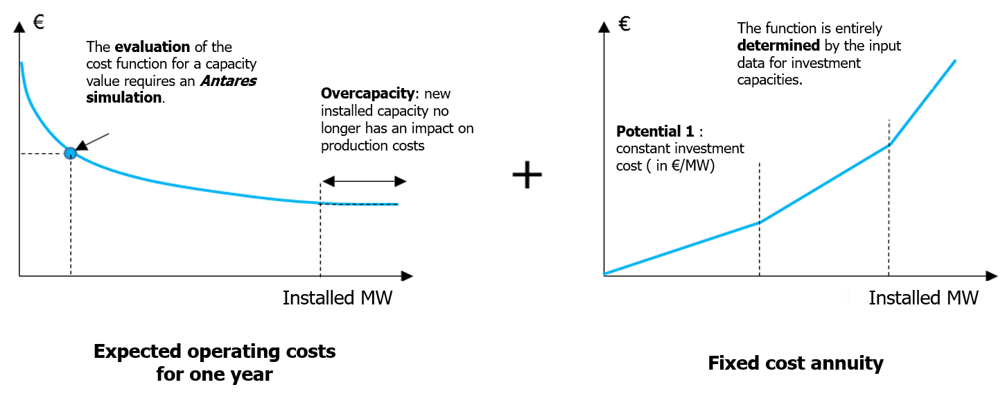
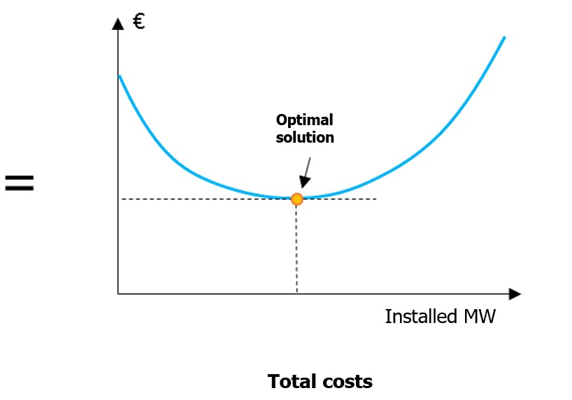
Figure 1 – Objective function of the Antares-Xpansion optimization problem for one candidate.

The expected operating costs for one year decrease as installed capacities increase. New generation or transmission capacities indeed reduce the variable operating costs of the power system by substituting "expensive" generation (or penalty in case of unsupplied energy) with generation from a cheaper source. The marginal contribution of the investment on this component of the cost function is decreasing: the "first" installed MW have the most interesting economic potential and a greater impact on generation costs than the "last" installed MW, which have a lower economic utility, or even none in the case of overcapacity. Mathematically, these characteristics ensure that the expected operating cost is a convex function of the installed capacity.

In Antares-Xpansion, fixed-cost annuities are considered piecewise linear. Different potentials are defined, each of which is characterized by a fixed annuity in €/MW installed, and corresponds to one of the slopes of the function, see Figure 1. A particular case of this representation of fixed annuities is a fully linear function, therefore characterized by a single fixed cost (in €/MW installed).

The final cost result - which will be called the total cost later on - is a convex function. It therefore has a minimum solution plateau (see Figure 2) which in most (but not all) applications on real data sets is reduced to a single point (see Figure 1). In some cases, there are several points leading to the optimal cost. Antares-Xpansion looks for an optimal solution, i.e. the point that minimizes the total cost, or any point of the minimum plateau in the case of a so-called degenerate problem.

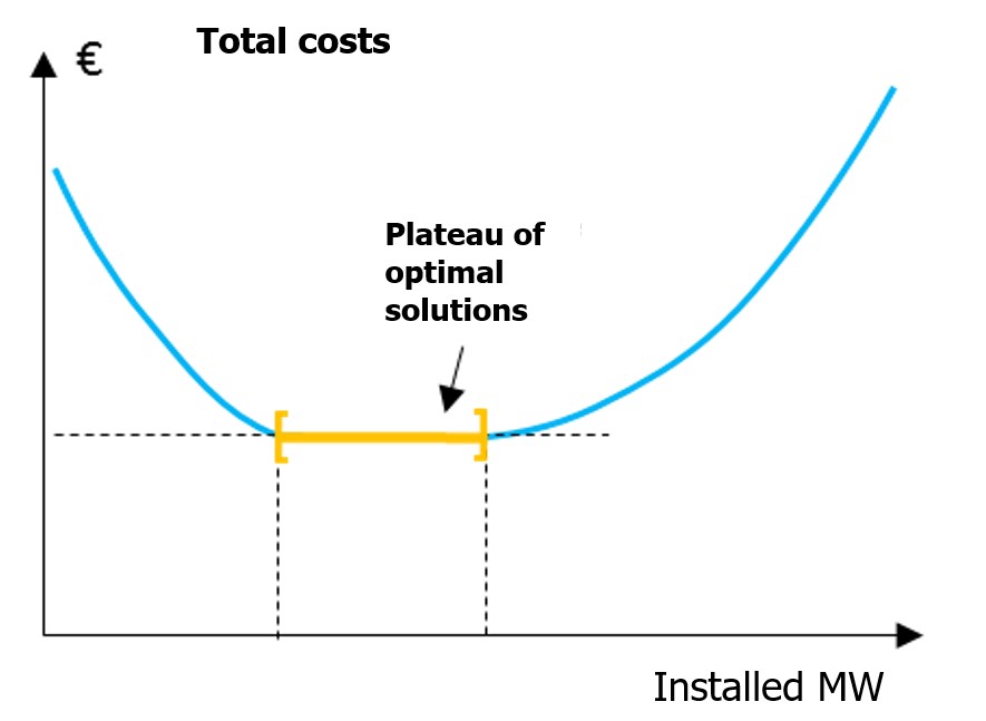
Figure 2 – Generic case (but uncommon in practical Antares-Xpansion cases) with a set of optimal solutions (a plateau).

Investment variables¶

The investment variables are the installed capacities (in MW) of the generation and/or transmission assets defined in the input of Antares-Xpansion as candidates for investment.

The cases shown in Figure 1 and Figure 2 contain only one investment variable. The search for the optimal solution is then carried out over the interval [0, available potential], bounded on the left by zero and on the right by the maximum available potential of the investment under consideration. The available potential is one of the input data of Antares-Xpansion.

In the more general case with several investment candidates, Antares-Xpansion determines one optimal investment combination, that is, one combination $(c_{1},c_{2},\ldots,c_{n})$ of the capacities of the $n$ investment candidates that minimizes the cost function.

The search for this optimal combination is done jointly (i.e. "at the same time") on the capacities of all investment candidates, and not candidate by candidate. By doing this, Antares-Xpansion is able to identify and assess the impact of synergies between structures - for example an A-B line which only becomes interesting once the B-C line is built - or of competitions - for example an A-B-C corridor parallel to another A-D-C corridor.

The definition of the investment variables in Antares-Xpansion is detailed in Define the candidates. For example, it may include:

Investable capacity values limited to a finite set rather than a whole interval. This allows to consider the following cases:
- The investment is made in unit steps of 200 MW and we wish to constrain the search of Antares-Xpansion to the discrete set {0 MW, 200 MW, 400 MW, 600 MW…}.
- Adopt an all-or-nothing approach in which only two choices are possible: not to invest or to invest up to an imposed unit capacity.
Antares-Xpansion can manage a mix of continuous investment variables, i.e. valid over the whole interval [0, maximum potential], and discrete variables, valid only over a finite set of values (see later).
Linear constraints between investable capacities. Linear constraints between variables can be defined in investment problems. For example, they may require the sum of the capacities of two investment candidates to be greater or less than a given limit.

Resolution with the Benders decomposition¶

The resolution method used by Antares-Xpansion - called Benders decomposition - is an iterative method, which for each iteration:

performs an Antares simulation to evaluate the expected annual operating costs of a combination of investments,
determines a new investment combination by solving a master problem in which the expected operating cost function is approximated by its derivatives computed at the previously tested investment combinations. These derivatives are also called Bender cuts.

A mathematical formulation of the optimization problem solved by Antares-Xpansion as well as details on the Benders decomposition method ar given in Mathematical formulation of the investment problem.

Notes on the computation time¶

The Benders decomposition method has been shown to converge towards the optimal solution of the investment problem described above and is also commonly used to solve large stochastic problems. The number of iterations required to reach the optimum strongly depends on the structure of the problem and on the variants/algorithmic parameters used. In general, it strongly increases with the number of defined investment variables, see Table 1.

Number of investment candidates	Order of magnitude of the number of iterations
5	10
10	40
25	100
50	300
100	800

Table 1 - Order of magnitude of the number of iterations required to reach the optimum with Antares-Xpansion v0.12.

Each iteration of the Antares-Xpansion algorithm includes an Antares simulation. However, the simulation of "operational" studies of several tens of nodes and with several hundred Monte-Carlo scenarios (TYNDP, Generation adequacy report on the electricity supply-demand, etc.) requires a significant amount of computing time, sometimes several hours. The search for the optimal solution to the problem solved by Antares-Xpansion can therefore be relatively long, and in some cases requires a simplification of the problem being solved.